a high-level algorithms expert will provide a brief overview of the evolution of neural networks and discuss the latest approaches in the field.
Neural networks and deep learning technologies underpin most of the advanced intelligent applications today. In this article, Dr. Sun Fei (Danfeng), a high-level algorithms expert from Alibaba's Search Department, will provide a brief overview of the evolution of neural networks and discuss the latest approaches in the field. The article is primarily centered on the following five items:
- The Evolution of Neural Networks
- Sensor Models
- Feed-forward Neural Networks
- Back-propagation
- Deep Learning Basics
1. The Evolution of Neural Networks
Before we dive into the historical development of neural networks, let's first introduce the concept of a neural network. A neural network is primarily a computing model that simulates the workings of the human brain at a simplified level. This type of model uses a large number of computational neurons which connect via layers of weighted connections. Each layer of neurons is capable of performing large-scale parallel computing and passing information between them.
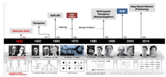
The timeline below shows the evolution of neural networks:
The origin of neural networks goes back to even before the development of computing itself, with the first neural networks appearing in the 1940s. We will go through a bit of history to help everyone gain a better understanding of the basics of neural networks.
The first generation of neural network neurons worked as verifiers. The designers of these neurons just wanted to confirm that they could build neural networks for computation. These networks cannot be used for training or learning; they simply acted as logic gate circuits. Their input and output was binary and weights were predefined.
The second phase of neural network development came about in the 1950s and 1960s. This involved Roseblatt's seminal work on sensor models and Herbert's work on learning principles.
2. Sensor Models
Sensor models and the neuron models as we mentioned above were similar but had some key differences. The activation algorithm in a sensor model can be either a break algorithm or a sigmoid algorithm, and its input can be a real number vector instead of the binary vectors used by the neuron model. Unlike the neuron model, the sensor model is capable of learning. Next, we will talk about some of the special characteristics of the sensor model.
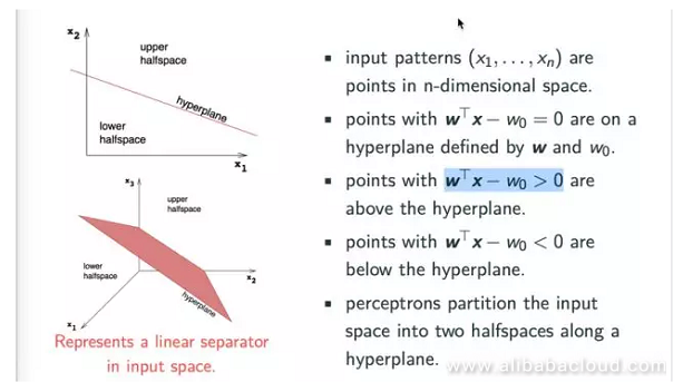
We can think of the input value (x1..., xn) as a coordinate in N dimensional space, while wTx-w0 = 0 is a hyperplane in N dimensional space. Obviously, if wTx-w0 < 0, then the point falls below the hyperplane, while if wTx-w0 > 0, then the point falls above the hyperplane.
The sensor model corresponds to the hyperplane of a classifier and is capable of separating different types of points in N dimensional space. Looking at the figure below, we can see that the sensor model is a linear classifier.
The sensor model is capable of easily performing classification for basic logical operations like AND, OR, and NOT.
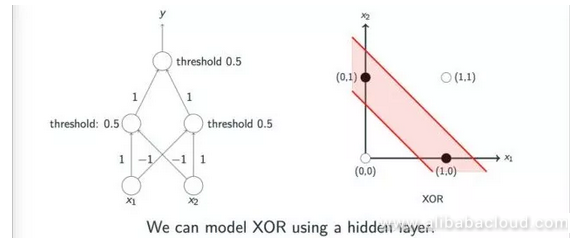
Can we classify all logical operations through the sensor model? The answer is, of course not. For example, Exclusive OR operations are very difficult to classify through a single linear sensor model, which is one of the main reasons that neural networks quickly entered a low point in development soon after the first peak. Several authors, including Minsky, discussed this problem on the topic of sensor models. However, a lot of people misunderstood the authors on this subject.
In reality, authors like Minsky pointed out that one could implement Exclusive OR operations through multiple layers of sensor models; however, since the academic world lacked effective methods to study multi-layer sensor models at the time, the development of neural networks dipped into its first low point.
The figure below shows intuitively how multiple layers of sensor models can achieve Exclusive OR operations:
3. Feed-Forward Neural Networks
Entering into the 1980s, due to the expressive ability of sensor model neural networks being limited to linear classification tasks, the development of neural networks began to enter the phase of multi-layered sensors. A classic multi-layered neural network is a feed-forward neural network.
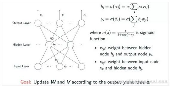
We can see from the figure below that it involves an input layer, a hidden layer with an undefined number of nodes, and an output layer.
We can express any logical operation by a multi-layer sensor model, but this introduces the issue of weighted learning between the three layers. When xk is transferred from the input layer to the weighted vkj on the hidden layer and then passed through an activation algorithm like sigmoid, then we can retrieve the corresponding value hj from the hidden layer. Likewise, we can use a similar operation to derive the yi node value from the output layer using the hj value. For learning, we need the weighted information from the w and v matrices so that we can finally obtain the estimated value y and the actual value d.
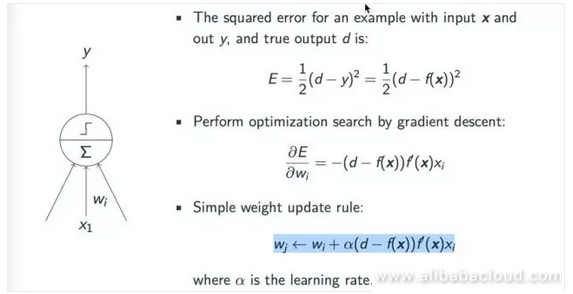
If you have a basic understanding of machine learning, you will understand why we use a gradient descent to learn a model. The principle behind applying a gradient descent to the sensor model is fairly simple, as we can see from the below figure. First, we have to determine the model's loss.
The example uses a square root loss and seeks to close the gap between the simulated value y and the real value d. For the sake of convenient computing, in most situations, we use the root relationship E = 1/2 (d-y)^2 = 1/2 (d-f(x))^2.
According to the gradient descent principle, the rate of the weighting update cycle is: wj ← wi + α(d − f(x))f′(x)xi, where α is the rate of learning which we can adjust manually.
4. Back-Propagation
How do we learn all of the parameters in a multilayer feed-forward neural network? The parameters for the top layer are very easy to obtain. One can achieve the parameters by comparing the difference between the estimated and real values output by the computing model and using the gradient descent principles to obtain the parameter results. The problem comes when we try to obtain parameters from the hidden layer. Even though we can compute the output from the model, we have no way of knowing what the expected value is, so we have no way of effectively training a multi-layer neural network. This issue plagued researchers for a long time, leading to the lack of development of neural networks after the 1960s.
Later, in the 70s, a number of scientists independently introduced the idea of a back-propagation algorithm. The basic idea behind this type of algorithm is actually quite simple. Even though at the time there was no way to update according to the expected value from the hidden layer, one could update the weights between the hidden and other layers via errors passed from the hidden layer. When computing a gradient, since all of the nodes in the hidden layer are related to multiple nodes on the output layer, so all of the layers on the previous layers are accumulated and processed together.
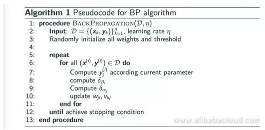
Another advantage of back-propagation is that we can perform gradients and weighting of nodes on the same layer at the same time since they are unrelated. We can express the entire process of back-propagation in pseudocode as below:
Next, let's talk about some of the other characteristics of a back-propagation neural network. A back-propagation is actually a chain rule. It can easily generalize any computation that has a map. According to the gradient function, we can use a back-propagation neural network to produce a local optimized solution, but not a global optimized solution. However, from a general perspective, the result produced by a back-propagation algorithm is usually a satisfactorily optimized solution. The figure below is an intuitive representation of a back-propagation algorithm:
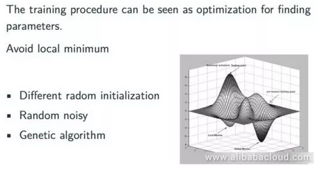
Under most circumstances, a back-propagation neural network will find the smallest possible value within scope; however, if we leave that scope we may find an even better value. In actual application, there are a number of simple and effective ways to address this kind of issue, for example, we can try different randomized initialization methods. Moreover, in practice, among the models frequently used in the field of modern deep learning, the method of initialization has significant influence on the final result. Another method of forcing the model to leave the optimized scope is to introduce random noises during training or use a hereditary algorithm to prevent the training model from stopping at an un-ideal optimized position.
A back-propagation neural network is an excellent model of machine learning, and when speaking about machine learning, we can't help but notice a basic issue that's frequently encountered throughout the process of machine learning, that is the issue of overfitting. A common manifestation of overfitting is that during training, even when the loss of the model constantly drops, the loss and error in the test group rises. There are two typical methods to avoid overfitting:
- Early stopping: we can separate a validation group ahead of time, and run it against this already verified group during training. We can then observe the loss of the model and, if the loss has already stopped dropping in the verification group but is still dropping in the training group, then we can stop the training early to prevent overfitting.
- Regularization: we can add rules to the weights within the neural network. The dropout method, which is popular these days, involves randomly dropping some nodes or sides. This method, which we can consider as a form of regularization, is extremely effective at preventing overfitting.
Even though neural networks were very popular during the 1980s, they, unfortunately, entered another low point in development in the 1990s. A number of factors contributed to this low point. For example, the Support Vector Machines, which were a popular model in the 1990s, took the stage at all kinds of major conferences and found application in a variety of fields. Support Vector Machines have an excellent statistical learning theory and are easy to intuitively understand. They are also very effective and produce near-ideal results.
Amidst this shift, the rise of the statistical learning theory behind Support Vector Machines applied no small amount of pressure to the development of neural networks. On the other hand, from the perspective of neural networks themselves, even though you can use back-propagation networks to train any neural network in theory, in actual application, we notice that as the number of layers in the neural network increases, the difficulty of training the network increases exponentially. For example, in the beginning of the 1990s, people noticed that in a neural network with a relatively large number of layers, it was common to see gradient loss or gradient explosion.
A simple example of gradient loss, for example, would be where each layer in a neural network is a sigmoid structure layer, therefore its loss during back-propagation is chained into a sigmoid gradient. When a series of elements are strung together, then if one of the gradients is very small, the gradient will then become smaller and smaller. In reality, after propagating one or two layers, this gradient disappears. Gradient loss leads to the parameters in deep layers to stop changing, making it very difficult to get meaningful results. This is one of the reasons that a multi-layer neural network can be very difficult to train.
The academic world has studied this issue in-depth, and come to the conclusion that the easiest way to handle it is by changing the activation algorithm. In the beginning, we tried to use a Rectified activation algorithm since the sigmoid algorithm is an index method which can easily bring about the issue of gradient loss. Rectified, on the other hand, replaces the sigmoid function and replaces max (0,x). From the figure below we can see that the gradient for estimates above 0 is 1, which prevents the issue of gradient disappearance. However, when the estimate is lower than 0, we can see that the gradient is 0 again, so the ReLU algorithm must be imperfect. Later, a number of improved algorithms came out, including Leaky ReLU and Parametric Rectifier (PReLU). When the estimate x is smaller than 0, we can convert it to a coefficient like 0.01 or α to prevent it from actually being 0.

With the development of neural networks, we later came up with a number of methods that solve the issue of passing gradients on a structural level. For example, the Metamodel, LSTM model, and modern image analysis use a number of cross-layer linking methods to more easily propagate gradients.
5. Deep Learning Basics
From the second low point in development in the 1990s to 2006, neural networks once again entered the consciousness of the masses, this time in even more force than before. A monumental occurrence during this rise of neural networks was the two theses on multi-layer neural networks (now called “deep learning”) submitted by Hinton in a number of places including Salahundinov.
One of these theses solved the issue of setting initialization values for neural networks. The solution, put simply, is to consider the input value as x, and the output value as decoded x, then through this method find a better initialization point. The other thesis raised a method of quickly training a deep neural network. Actually, there are a number of factors contributing to the modern popularity of neural networks, for example, the enormous growth in computing resources and availability of data. In the 1980s, it was very difficult to train a large scale neural network due to the lack of data and computing resources.
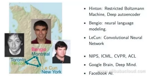
The early rise of neural networks was driven by three monumental figures, namely Hinton, Bengio, and LeCun. Hinton's main accomplishment was in the Restricted Boltzmann Machine and Deep Autoencoder. Bengio's major contribution was a series of breakthroughs in using the metamodel for deep learning. This was also the first field in which deep learning experienced a major breakthrough.
In 2013, language modeling, based on the metamodel, was already capable of outperforming even the most effective method at the time, the probability model. The main accomplishment of LeCun was research related to CNN. The primary appearance of deep learning was in a number of major summits like NIPS, ICML, CVPR, ACL, where it attracted no small amount of attention. This included the appearance of Google Brain, Deep Mind, and Facebook AI, which all placed the center of their research on the field of deep learning.
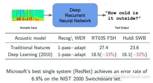
The first breakthrough to come about after deep learning entered the consciousness of the masses was in the field of speech recognition. Before we began using deep learning, models were all trained on previously defined statistical databases. In 2010, Microsoft used a deep learning neural network for speech recognition. We can see from the figure below that two error indicators both dropped by 2/3, an obvious improvement. Based on the newest ResNet technology, Microsoft has already reduced this indicator to 6.9%, with improvements coming year by year.
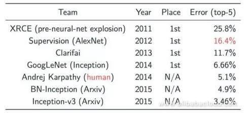
In the field of image classification, the CNN model experienced a major breakthrough in the form of ImageNet in 2012. In ImageNet, the Image classification is tested using a massive data collection and then sorted into 1000 types. Before the application of deep learning, the best error rate for image classification system was 25.8% (in 2011), which came down to a mere 10%, thanks to the work done by Hinton and his students in 2012 using CNN.
From the graph, we can see that since 2012, this indicator has experienced a major breakthrough each year, all of which have been achieved using the CNN model.
These massive achievements owe in large part to the multi-layered structure of modern systems, as they allow for independent learning and the ability to express data through a layered abstraction structure. The abstracted features can be applied to a variety of tasks, contributing significantly to the current popularity of deep learning.
Next, we will introduce two classic and common types of deep learning neural networks: One is the Convolutional Neural Network (CNN), and the other is the Recurrent Neural Network
Convolutional Neural Networks
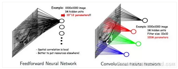
There are two core concepts to Convolutional Neural Networks. One is convolution and the other is pooling. At this point, some may ask why we don't simply use feed-forward neural networks rather than CNN. Taking a 1000x1000 image, for example, a neural network would have 1 million nodes on the hidden layer. A feed-forward neural network, then, would have 10^12 parameters. At this point, it's nearly impossible for the system to learn since it would require an absolutely massive number of estimations.
However, a large number of images have characteristics like this. If we use CNN to classify images, then because of the concept of convolution, each node on the hidden layer only needs to connect and scan the features of one location of the image. If each node on the hidden layer connects to 10*10 estimations, then the final number of parameters is 100 million, and if the local parameters accessed by multiple hidden layers can be shared, then the number of parameters is decreased significantly.
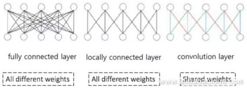
Looking at the image below, the difference between feed-forward neural networks and CNN is obviously massive. The models in the image are, from left to right, fully connected, normal, feed-forward, fully connected feed-forward, and CNN modeled neural networks. We can see that the connection weight parameters of nodes on the hidden layer of a CNN neural network can be shared.
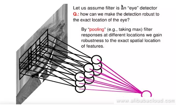
Another operation is pooling. A CNN will, on the foundation of the principle of convolution, form a hidden layer in the middle, namely the pooling layer. The most common pooling method is Max Pooling, wherein nodes on the hidden layer choose the largest output value. Because multiple kernels are pooling, we get multiple hidden layer nodes in the middle.
What is the benefit? First of all, pooling further reduces the number of parameters, and secondly, it provides a certain amount of translation invariance. As shown in the image, if one of the nine nodes shown in the image were to experience translation, then the node produced on the pooling layer would remain unchanged.
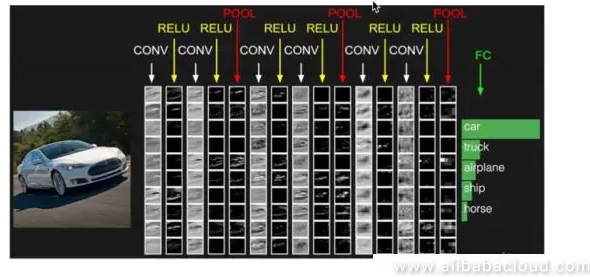
These two characteristics of CNN have made it popular in the field of image processing, and it has become a standard in the field of image processing. The example of the visualized car below is a great example of the application of CNN in the field of image classification. After entering the original image of the car into the CNN model, we can pass some simple and rough features like edges and points through the convolution and ReLU activation layer. We can intuitively see that the closer they are to the output image from the uppermost output layer, the closer they are to the contours of a car. This process will finally retrieve a hidden layer representation and connect it to the classification layer, after which it will receive a classification for the image, like the car, truck, airplane, ship, and horse shown in the image.
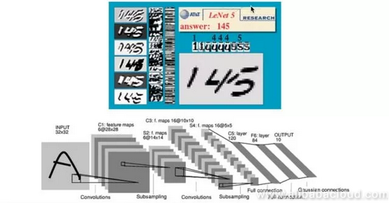
The image below is a neural network used in the early days by LeCun and other researchers in the field of handwriting recognition. This network found application in the US postal system in the 1990s. Interested readers can log into LeCun's website to see the dynamic process of handwriting recognition.
While CNN has become incredibly popular in the field of image recognition, it has also become instrumental in text recognition over the past two years. For example, CNN is currently the basis of the most optimal solution for text classification. In terms of determining the class of a piece of text, all one really needs to do is look for indications from keywords in the text, which is a task that is well suited to the CNN model.
CNN has widespread real-world applications, for example in investigations, self-driving cars, Segmentation, and Neural Style. Neural Style is a fascinating application. For example, there is a popular app in the App Store called Prisma, which allows users to upload an image and convert it into a different style. For example, it can be converted to the style of Van Goh's Starry Night. This process relies heavily on CNN.
Recursive Neural Networks
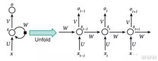
As for the foundational principles behind recursive neural networks, we can see from the image below that the output from such a network relies not only on output x but the status of the hidden layer, which is updated according to the previous input x. The expanded image shows the entire process. The hidden layer from the first input is S(t-1), which influences the next input, X(t). The main advantage of the recursive neural network model is that we can use it in sequential data operations like text, language, and speech where the state of the current data is influenced by previous data states. This type of data is very difficult to handle using a feed-forward neural network.
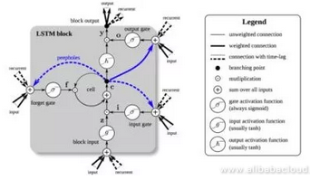
Speaking of recursive neural networks, we would be remiss not to bring up the LSTM model we mentioned earlier. LSTM is not actually a complete neural network. Simply put, it is the result of an RNN node that has undergone complex processing. An LSTM has three gates, namely the input gate, the regret gate, and the output gate.
Each of these gates is used to process the data in a cell and determine whether or not the data in the cell should be input, regretted, or output.
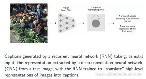
Finally, let's talk a bit about a cross-discipline application of neural networks which is gaining widespread acceptance. This application involves converting an image into a text description of the image or a title describing it. We can describe the specific implementation process by using a CNN model first to extract information about the image and produce a vector representation. Later on, we can pass that vector as input to an already trained recursive neural network to produce the description of the image.
Summary
In this article, we talked about the evolution of neural networks and introduced several basic concepts and approaches in this field.
Source: https://dzone.com/articles/all-you-need-to-know-about-neural-networks-part-2